Displaying Detected Peaks

PyMassSpec-Plot also allows for detected peaks to marked on a TIC plot.

First, setup the paths to the datafiles and the output directory, then import JCAMP_reader() and build_intensity_matrix.

In [1]:

from domdf_python_tools.paths import PathPlus

cwd = PathPlus(".").resolve()
data_directory = PathPlus(".").resolve().parent.parent / "datafiles"
# Change this if the data files are stored in a different location

output_directory = cwd / "output"

from pyms.GCMS.IO.JCAMP import JCAMP_reader
from pyms.IntensityMatrix import build_intensity_matrix

Read the raw data files, extract the TIC and build the IntensityMatrix.

In [2]:

jcamp_file = data_directory / "gc01_0812_066.jdx"
data = JCAMP_reader(jcamp_file)
data.trim("500s", "2000s")
tic = data.tic
im = build_intensity_matrix(data)

 -> Reading JCAMP file '/home/runner/work/PyMassSpec-Plot/PyMassSpec-Plot/datafiles/gc01_0812_066.jdx'
Trimming data to between 520 and 4517 scans

Perform pre-filtering and peak detection. For more information on detecting peaks see the Peak detection and representation chapter of the PyMassSpec documentation.

In [3]:

from pyms.Noise.SavitzkyGolay import savitzky_golay
from pyms.TopHat import tophat
from pyms.BillerBiemann import BillerBiemann, rel_threshold, num_ions_threshold

n_scan, n_mz = im.size

for ii in range(n_mz):
    ic = im.get_ic_at_index(ii)
    ic_smooth = savitzky_golay(ic)
    ic_bc = tophat(ic_smooth, struct="1.5m")
    im.set_ic_at_index(ii, ic_bc)

# Detect Peaks
peak_list = BillerBiemann(im, points=9, scans=2)

print("Number of peaks found: ", len(peak_list))

# Filter the peak list, first by removing all intensities in a peak less than a
# given relative threshold, then by removing all peaks that have less than a
# given number of ions above a given value

pl = rel_threshold(peak_list, percent=2)
new_peak_list = num_ions_threshold(pl, n=3, cutoff=10000)

print("Number of filtered peaks: ", len(new_peak_list))

Number of peaks found:  1467
Number of filtered peaks:  72

Get Ion Chromatograms for 4 separate m/z channels.

In [4]:

ic191 = im.get_ic_at_mass(191)
ic73 = im.get_ic_at_mass(73)
ic57 = im.get_ic_at_mass(57)
ic55 = im.get_ic_at_mass(55)

Import matplotlib, and the plot_ic() and plot_peaks() functions.

In [5]:

import matplotlib.pyplot as plt
from pyms.Display import plot_ic, plot_peaks

Create a subplot, and plot the TIC.

In [6]:

fig, ax = plt.subplots(1, 1, figsize=(8, 5))

# Plot the ICs
plot_ic(ax, tic, label="TIC")
plot_ic(ax, ic191, label="m/z 191")
plot_ic(ax, ic73, label="m/z 73")
plot_ic(ax, ic57, label="m/z 57")
plot_ic(ax, ic55, label="m/z 55")

# Plot the peaks
plot_peaks(ax, new_peak_list)

# Set the title
ax.set_title('TIC, ICs, and PyMS Detected Peaks')

# Add the legend
plt.legend()

plt.show()

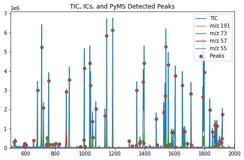
The function plot_peaks() adds the PyMassSpec detected peaks to the figure.

The function pyms.Peak.List.IO.store_peaks() can be used to store the peaks, which can be loaded back with pyms.Peak.List.IO.load_peaks() for later display.

When not running in Jupyter Notebook, the plot may appear in a separate window like the one shown in Fig. 4.

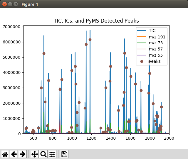
Fig. 4 Graphics window displayed by the Displaying_Detected_Peaks.py script

Note

This example is in demo/jupyter/Displaying_Detected_Peaks.ipynb and demo/scripts/Displaying_Detected_Peaks.py.