Displaying a TIC

First, setup the paths to the datafiles and the output directory, then import JCAMP_reader().

In [1]:

from domdf_python_tools.paths import PathPlus

cwd = PathPlus(".").resolve()
data_directory = PathPlus(".").resolve().parent.parent / "datafiles"
# Change this if the data files are stored in a different location

output_directory = cwd / "output"

from pyms.GCMS.IO.JCAMP import JCAMP_reader

Read the raw data files and extract the TIC.

In [2]:

jcamp_file = data_directory / "gc01_0812_066.jdx"
data = JCAMP_reader(jcamp_file)
tic = data.tic

-> Reading JCAMP file '/home/runner/work/PyMassSpec-Plot/PyMassSpec-Plot/datafiles/gc01_0812_066.jdx'

Import matplotlib and the plot_ic() function, create a subplot, and plot the TIC:

In [3]:

import matplotlib.pyplot as plt
from pymassspec_plot import plot_ic

fig, ax = plt.subplots(1, 1, figsize=(8, 5))

# Plot the TIC
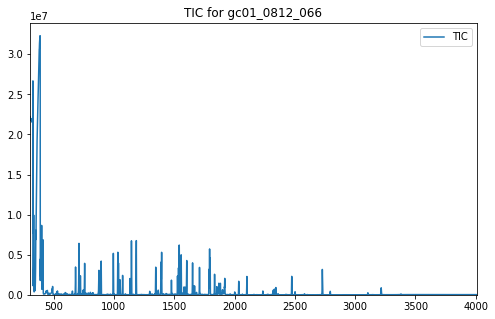
plot_ic(ax, tic, label="TIC")

# Set the title
ax.set_title("TIC for gc01_0812_066")

# Add the legend
plt.legend()

plt.show()

In addition to the TIC, other arguments may be passed to plot_ic(). These can adjust the line colour or the text of the legend entry. See matplotlib.lines.Line2D for a full list of the possible arguments.

An IonChromatogram can be plotted in the same manner as the TIC in the example above.

When not running in Jupyter Notebook, the plot may appear in a separate window like the one shown in Fig. 1.

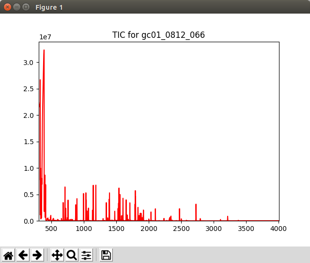
Fig. 1 Graphics window displayed by the Displaying_TIC.py script

Note

This example is in demo/jupyter/Displaying_TIC.ipynb and demo/scripts/Displaying_TIC.py.